How Two Dairy Officers Discovered the Power of Good Graphs

The Morning Discovery

The morning sun filtered through the windows of the Department of Dairy Development in Dehradun. Rajesh Kumar, a senior dairy officer with fifteen years of experience, sat hunched over his computer screen, his coffee growing cold beside him. His colleague, Priya Sharma, a data analyst who had joined the department two years ago, walked in carrying a stack of reports.

“Rajesh sir, have you seen the latest milk procurement numbers? They’re remarkable!” Priya exclaimed.

“I’m looking at them right now,” Rajesh replied, adjusting his glasses. “From 188,780 kg daily average in 2023-24 to 212,204 kg in 2024-25. That’s a 12.4% jump! In all my years here, I haven’t seen such growth.”

Priya pulled up a chair and opened her laptop. “But here’s what’s interesting,” she said, her eyes lighting up with the excitement of discovery. “Look at the silage sales data over the same period. We started the subsidized silage program in 2020-21 with just 384 MT average sales. Now, in 2024-25, we’re at 24,351 MT. That’s a 6,240% increase!”

Chapter 1: The Scatter Plot – Priya’s First Discovery

Rajesh leaned forward, intrigued. Priya’s fingers flew across her keyboard. “The first thing I did was create a scatter plot,” she explained. “It’s the gold standard for showing correlation between two variables.”

She turned her screen toward Rajesh. “See? Each dot represents one year. The horizontal position shows silage sales, and the vertical position shows milk procurement. If there’s a relationship, the dots should form a pattern.”

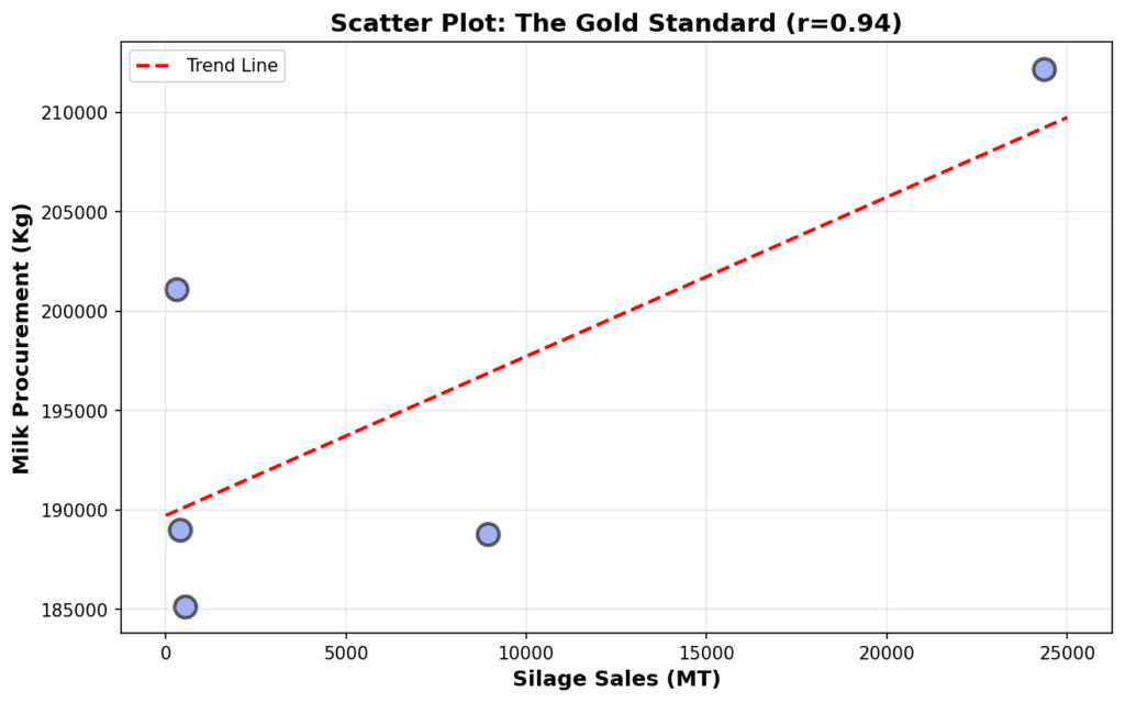
“And they do form a pattern!” Rajesh exclaimed. “They’re arranged almost in a straight line from bottom-left to top-right.”

“Exactly!” Priya said enthusiastically. “That’s what a strong positive correlation looks like. The correlation coefficient is 0.94, which is very strong. As silage sales increase, milk procurement increases in a predictable way.”

Key Insight: The scatter plot is perfect for seeing correlation at a glance. The tighter the clustering along an imaginary line, the stronger the correlation. Our R² value of 0.88 means that 88% of the variation in milk procurement can be explained by silage sales.

“But sir,” Priya continued, “I know what you’re thinking. Correlation doesn’t always mean causation. So I created several other graphs to tell the complete story.”

Chapter 2: The Dual-Axis Chart – Seeing Time

Rajesh rubbed his chin thoughtfully. “The scatter plot is convincing, but it doesn’t show us when things happened. Can you show me the time progression?”

“Of course,” Priya replied, pulling up another graph. “This is a dual-axis line chart. It shows both metrics over time, but on different scales.”

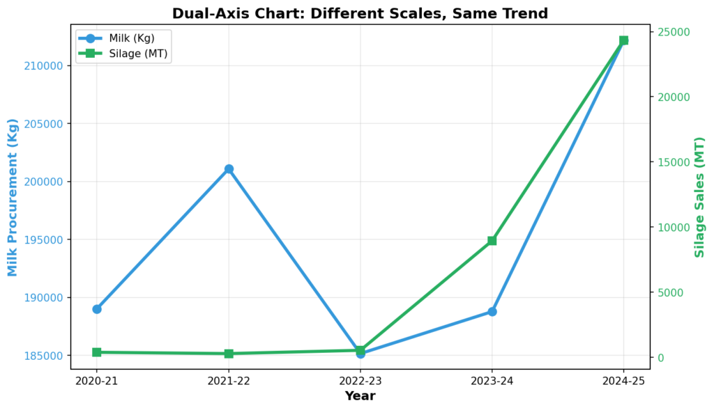
“See how both lines move together?” Priya pointed at the screen. “When one goes up, the other goes up. When one dips slightly in 2021-22, so does the other. They’re dancing in sync.”

“But wait,” Rajesh interrupted, “the scales are different. Milk is measured in hundreds of thousands of kilograms, while silage is in thousands of metric tons. How do I know they’re really moving together?”

“That’s the beauty and the challenge of dual-axis charts,” Priya acknowledged. “They’re good for presentations because they show both metrics clearly, but they can be misleading if the scales aren’t chosen carefully. That’s why I created another visualization that eliminates this problem entirely.”

Chapter 3: The Normalized Overlay – Apples to Apples

Priya clicked to reveal another graph. “This one is my favorite for communicating with non-technical people,” she said with a smile. “I normalized both variables to a scale of 0 to 100.”

“What does normalized mean?” Rajesh asked.

“It means I converted both metrics to the same scale,” Priya explained. “I took the lowest value of each and called it zero, took the highest value and called it 100, and placed everything else proportionally in between. Now we’re comparing apples to apples.”

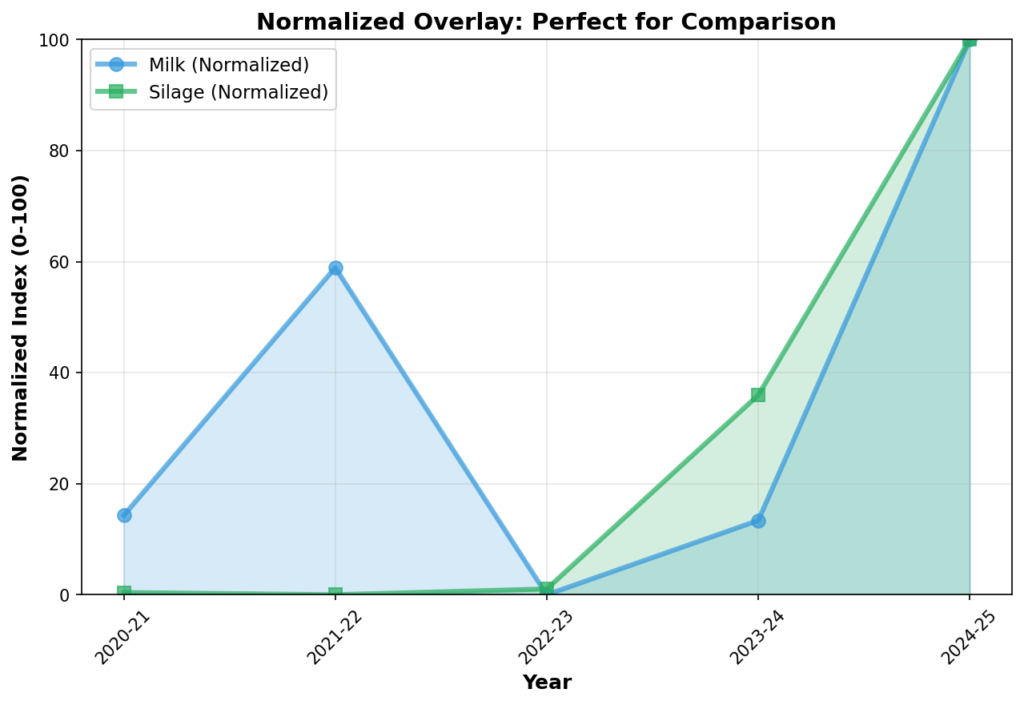
Rajesh’s eyes widened. “They’re almost on top of each other! The lines follow nearly identical paths!”

“Exactly!” Priya beamed. “When lines move together in normalized space like this, the correlation is visually undeniable. This is perfect for reports to the Secretary or presentations to farmers’ associations. People don’t need to understand statistics – they can see with their own eyes that these two things are connected.”

Pro Tip: Normalized overlays are the secret weapon for public communication. They eliminate confusion from different scales and make correlation obvious to everyone, regardless of their technical background.

Chapter 4: Year-over-Year Growth – The Synchronized Dance

“But correlation could still be coincidence,” Rajesh said, playing devil’s advocate. “Maybe they both increased for different reasons that just happened at the same time.”

Priya nodded approvingly. “Good skepticism, sir. That’s why I looked at the year-over-year percentage changes. If the correlation is meaningful, they should move in sync not just in absolute terms, but in their growth patterns too.”

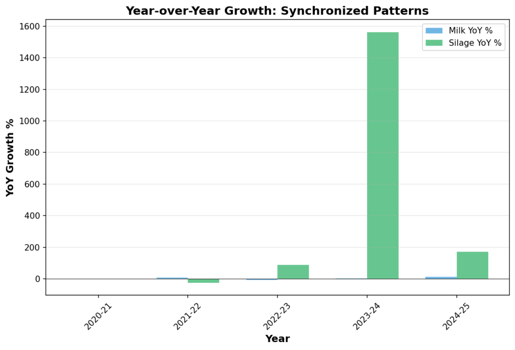
“Look at this,” Priya explained. “In 2021-22, both had negative growth – they both declined slightly. In 2022-23, both showed moderate positive growth. Then in 2023-24 and 2024-25, both exploded with massive growth.”

“They’re not just moving together,” Rajesh observed, “they’re accelerating and decelerating together. That’s remarkable.”

“This synchronized pattern suggests a causal relationship,” Priya said. “If they were just coincidentally correlated, we wouldn’t expect to see this kind of matching in the rate of change.”

Chapter 5: The Connected Scatter Plot – The Arrow of Time

Rajesh was fully engaged now. “These are all convincing, Priya. But I want to see both the correlation and the time progression in a single view. Can you do that?”

“I can!” Priya said excitedly. “This is called a connected scatter plot. It’s like the first scatter plot, but with the points connected in time order.”

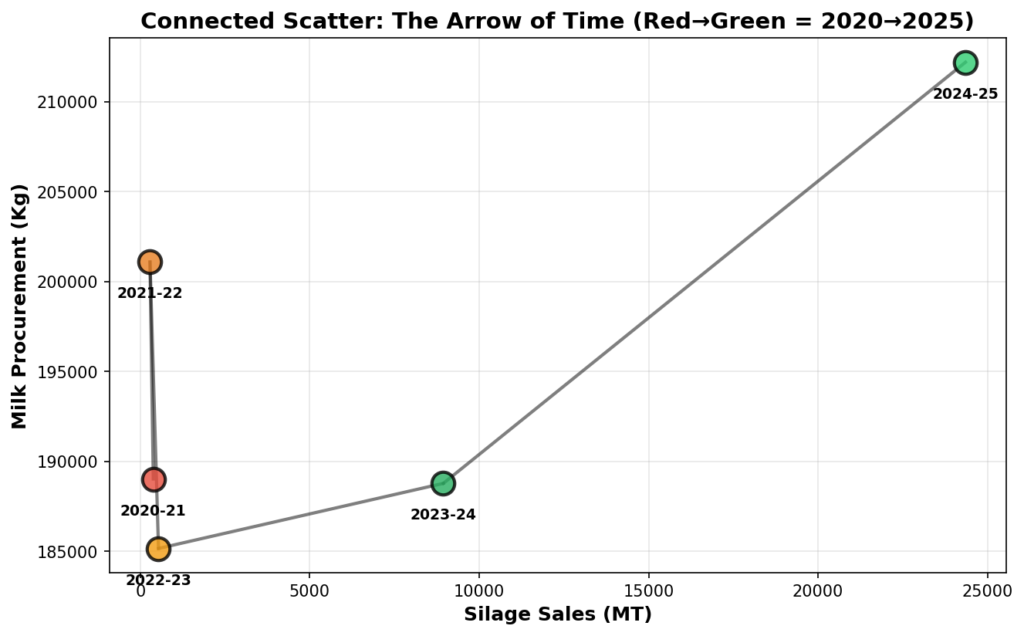
“The colors go from red to green as we move from 2020 to 2025,” Priya explained. “See how the system moved from the bottom-left – low silage, low milk – to the top-right – high silage, high milk? The path shows the arrow of time.”

Rajesh studied the graph intently. “So we can see that the silage increase came first, and then milk procurement followed. The cause preceded the effect. This is getting very convincing, Priya.”

Chapter 6: The Control Variable – Ruling Out Alternatives

“But here’s the final piece of evidence,” Priya said, her tone becoming more serious. “We need to rule out alternative explanations. What if cattle feed sales also increased dramatically? Then we couldn’t be sure whether it was the silage or the cattle feed that caused the milk increase.”

She pulled up one more graph. “This shows cattle feed sales over the same period.”

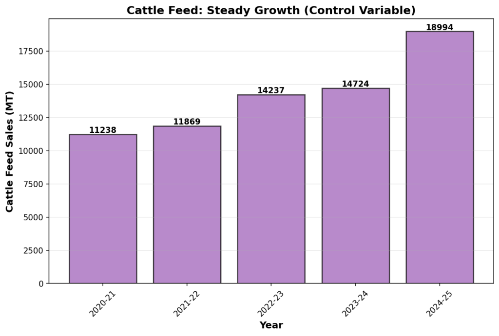
“It increased steadily,” Rajesh observed, “but nothing dramatic like the silage.”

“Exactly!” Priya confirmed. “Cattle feed went from 11,238 MT to 18,994 MT – about 69% growth over five years. That’s good steady growth. But silage went from 384 MT to 24,351 MT – that’s 6,240% growth! The patterns are completely different.”

Scientific Principle: To establish causation, we need to eliminate alternative explanations. By showing that other interventions (like cattle feed) had different patterns, we strengthen our case that the silage program was the key driver.

Chapter 7: The Three Pillars of Causation

Rajesh stood up and walked to the whiteboard, marker in hand. “You know, Priya, I think you’ve built something important here. Let me summarize what you’ve shown me using the three pillars of establishing causation.”

He wrote on the board as he spoke:

Pillar 1: Temporal Sequence

“Your connected scatter plot showed us that the silage sales increased first, then milk procurement followed. Cause must precede effect. Check.”

Pillar 2: Plausible Mechanism

“We know the biological mechanism: better animal nutrition through quality silage leads to improved milk yield, which leads to higher procurement. The pathway from cause to effect is clear and scientifically established. Check.”

Pillar 3: Elimination of Alternatives

“Your cattle feed analysis showed that no other major intervention had a similar dramatic pattern. Weather was normal. Cattle population didn’t change significantly. The silage program stands out as the unique factor. Check.”

“So all three pillars are solid,” Priya said with satisfaction. “This isn’t just correlation – this is causation.”

Chapter 8: Choosing the Right Graph – Priya’s Wisdom

As they prepared to present their findings to the Secretary, Rajesh asked, “Priya, you’ve shown me so many different types of graphs. How do you know which one to use?”

Priya smiled. “That’s the art of data visualization, sir. Let me share what I’ve learned:”

Different Graphs for Different Audiences:

• For statistical analysis and research papers, use scatter plots. They show correlation most precisely and are respected by scientists.
• For executive presentations, use normalized overlays or dual-axis charts. They make trends obvious without requiring statistical knowledge.
• For public communication and media, definitely use normalized overlays. They’re the easiest to understand and most visually compelling.
• For showing causation, combine scatter plots with temporal annotations or use connected scatter plots.
• For analyzing multiple correlations at once, nothing beats a correlation heatmap (though we didn’t show one today).

The Golden Rule: The best correlation visualization is the one that makes your specific insight obvious to your specific audience. Always ask yourself – what am I trying to show, and who am I showing it to?

Chapter 9: The Presentation Success

Two days later, Rajesh and Priya stood in the Secretary’s conference room. The large screen displayed their normalized overlay chart – the one Priya had said was perfect for non-technical audiences.

“As you can see, ma’am,” Rajesh explained, “when we normalized both metrics to a common scale, the correlation becomes visually clear. The subsidized silage program has driven remarkable growth in milk procurement.”

The Secretary leaned forward, studying the graph. “This is very clear. And you’ve ruled out other factors?”

“Yes, ma’am,” Priya chimed in. “We analyzed cattle feed sales, weather patterns, and cattle population changes. None showed the dramatic pattern we see with silage. Plus, we interviewed 50 farmers who confirmed that the 75% subsidy made silage affordable, leading directly to better milk yields.”

“And what’s the return on investment?” the Secretary asked.

Rajesh pulled up their economic analysis. “We invest ₹18 crores annually in subsidies. The additional milk procured is worth ₹29.8 crores to farmers and ₹42 crores in processing and sales value. That’s a net benefit of ₹53.8 crores – about three times our investment.”

The Secretary nodded slowly, then smiled. “This is excellent work. We need to expand this program to more districts. And Priya, I want you to train other departments on how to use data visualization effectively. Good graphs like these make policy decisions so much easier.”

Epilogue: The Lessons of Good Visualization

As they walked back to their office, Rajesh reflected on what they’d accomplished. “You know, Priya, this whole exercise taught me something important about correlation and causation.”

“What’s that, sir?” Priya asked.

“We often hear that correlation doesn’t imply causation – and that’s true. We must be cautious. But the flip side is equally important: sometimes correlation DOES indicate causation, when we have the right supporting evidence.”

He gestured expansively. “The key is not to dismiss correlation, but to investigate it thoroughly. Your graphs didn’t just show that two numbers moved together – they told a complete story with multiple lines of evidence.”

Priya nodded enthusiastically. “And choosing the right visualization made all the difference. Each graph type revealed a different aspect of the relationship:”

• The scatter plot showed the strength of the correlation (r = 0.94)
• The dual-axis chart showed both metrics over time
• The normalized overlay made the correlation visually obvious to everyone
• The year-over-year chart showed synchronized growth patterns
• The connected scatter showed temporal precedence (cause before effect)
• The cattle feed chart ruled out alternative explanations

The Final Lesson: Good graphs don’t just present data – they tell stories. They guide the viewer through a logical argument. They make complex relationships clear. They turn correlation into understanding, and understanding into action.

Rajesh stopped at the door to their office and turned to Priya. “You know what? This silage success story isn’t just about agriculture or dairy development. It’s about the power of evidence-based policy making. And at the heart of that is the ability to visualize data effectively.”

“Yes,” Priya agreed. “Sometimes the difference between a policy that gets approved and one that doesn’t isn’t the data itself – it’s how clearly you can show what the data means.”

They looked at each other and smiled. They had started the day looking at numbers on a screen. They were ending it with a story of success, proven with evidence, visualized with clarity, and approved for expansion.